Woodland genetic genealogy talk

I gave a talk as part of the Woodland (CA) Public Library Science & Society Discussion Series (Thurs once a month). The powerpoint of the slides is here: Woodland genetic genealogy slides [ppt], a pdf of the slides is here (but lacks the animations & gifs).

The discussion was a lot of fun, with many great questions. Thanks to Sudhir Vaikkattil for inviting me, and to Woodland Public Library for hosting the series, the discussion series future schedule is here.

If you’re interested in more information you can read my blog posts on the topic, or check out one of these great books on the topic

Screen Shot 2018-06-29 at 9.31.01 AM.png

Posted in genetic genealogy, personal genomics, popgen teaching | Leave a comment

Coop lab at PEGQ

Emily Josephs. Detecting polygenic adaptation in maize. 11:20am – 11:40am Mon, May 14

Erin Calfee. Methods for detecting selection in admixed populations. Short talk: 4:30pm – 4:35pm Mon, May 14. Poster (56M) 8:00pm – 9:00pm Mon, May 14

Doc Edge. Reconstructing the history of polygenic adaptation using local coalescent trees. Poster (324T) 8:00pm – 9:00pm Tue, May 15

Sivan Yair. Characterizing adaptive Neanderthal introgression using ancient and modern population genomic data. Poster (122M) 8:00pm – 9:00pm Mon, May 14

Nancy Chen. Tracking short-term evolution in a pedigreed wild population. 11:00am – 11:15am. Tue, May 15

Kristin Lee. Detecting signatures of convergent adaptation in population genomic data. 3:15pm – 3:30pm Tue, May 15

Vince Buffalo. “A temporal signal of linked selection.” 3:45pm – 4:00pm Tue, May 15 2nd Floor – Capitol Ballroom

Posted in cooplab, meetings | Leave a comment

How lucky was the genetic investigation in the Golden State Killer case?

Last week, police arrested Joseph DeAngelo as a suspect in case of the Golden State Killer, an infamous serial murderer and rapist whose case has been open for over forty years. The arrest is huge news in and of itself, but for people interested in the social uses of genetic data, the way in which DeAngelo was identified—using genetic genealogy & genetic data from crime-scene samples—was noteworthy. In this blog post, we discuss some of the genetics and math underlying the way in which he was identified (see also Henn et al). Because there’s been lots of discussion of the ethics of these approaches, we will not focus on that here; see here for a collection of links & news articles.

 The use of genetic data to identify suspects is not new. In the US, law enforcement makes extensive use of their CODIS (Combined DNA Index System) database—genetic searches against the database have aided almost 400,000 investigations since the mid-1990s. The CODIS database contains the genotypes of over 13 million people, most of whom have been convicted of a crime. The genetic information included about each person in the CODIS database is relatively sparse. Most of the profiles record genotypes at just 13 sites in the genome (since 2017, 20 sites have been genotyped). Because the CODIS sites are highly variable microsatellites, CODIS genotypes identify people nearly uniquely—they are sometimes called “DNA fingerprints” . (The CODIS markers reveal more than fingerprints do, though–they can reveal considerable ancestry information, can reveal close relatives, and in some cases, it’s possible to identify genome-wide genetic profiles that “match” a particular CODIS dataset well.)

 In a typical case in which law enforcement uses genetic data, the procedure is to genotype a crime-scene sample at the CODIS loci and look for a full or partial match against the CODIS database. If the sample came from a person who is in the CODIS database, he or she is likely to be identified. If there is no match, then the genetic search ends unless other information can be brought to bear.

 In the Golden State Killer case, genotyping the samples at the CODIS markers did not reveal a match—Joseph DeAngelo was apparently not included in the CODIS database. Nonetheless, the genetic search continued. Investigators apparently genotyped the crime scene sample at a genome-wide set of SNPs, or single-nucleotide polymorphisms. SNPs are the markers of choice for large consumer genetics services like Ancestry and 23andMe (as well as for genome-wide association studies [GWAS].) The police cannot access private databases like these—at least not without an extended legal process—but they do not have to. Many users upload their SNP data to third-party websites to perform advanced analyses or to search for matches with people tested by different companies.

 These SNP databases are growing rapidly. The plot below shows the number of users in each of a set of repositories over the last few years (plot from here). The largest databases—AncestryDNA and 23andMe—are private. But the fourth-largest—GEDmatch, which now has about 950,000 profiles—is an online service that searches for genetic matches with any user who uploads an appropriately formatted genotype file. That’s the one that police searched for DeAngelo.

 Investigators searched for the suspect’s profile by making a personal user account and uploading a genotype file created from the SNP data obtained from crime-scene samples. To do this, the investigators must have created a data file mimicking the SNP set and file format provided by some genetic genealogy company . There was no exact match in the GEDmatch database—indeed, investigators did not expect that DeAngelo would have uploaded his own data—but the trail was not yet cold. The police could still run a  search scanning the database for relatives of the suspect. If it is possible to identify a close relative, then the search for the suspect will be narrowed considerably, even if the suspect is not in the database. This is similar to the familial searching done using the CODIS database, which is legal in some States. (But it is imperfect, see work here and here from Rori Rohlfs and colleagues). However, in the CODIS database, familial search efficacy is limited to close relatives (usually parents and siblings, and more tenuously uncles/aunts/nieces/nephews and first cousins). Thirteen microsatellite markers’ worth of information is simply not enough to distinguish a distant cousin from an unrelated person. With the hundreds of thousands of markers on a typical SNP chip, familial searching is much more powerful—third cousins can be found most of the time, and many (but not all) fourth cousins can be found too. A sample set of profile matches from GEDmatch is shown below:

 Looking at SNP-based relative matches in GEDmatch, police found what they needed in the form of 10 to 20 likely relatives. These likely relatives represented third-to-fourth cousins of DeAngelo, most of whom he had probably never met. Using this genetic data, in combination with genealogical information about these relatives, the Golden State Killer investigation narrowed to one extended family, eventually honing in on DeAngelo himself.

 Geneticists and genetic genealogists have been using these techniques for some time; the GEDmatch database exists because genealogists wanted to share genomic resources to help identify relatives, allowing families to be reunited (see here). Widespread reporting of the method used to identify DeAngelo as the suspected Golden State Killer has inspired a surge of interest in genetic privacy (see here for a general review of topic). Though DeAngelo’s capture is widely celebrated, people are also understandably surprised that the decisions of third or fourth cousins can potentially expose one to surveillance. In this post, we explore some simple models to ask questions about the extent of surveillance that is possible using the methods employed in the Golden State Killer case.

 Two opposed phenomena govern the effectiveness of familial searches on genetic databases, one genealogical and one genetic. The genealogical phenomenon, which we could call “genealogical blowup”, is that the number of relatives one has at a specified degree of relatedness increases as the relatedness becomes more distant. For example, whereas a typical person may have one, two, or three siblings, he or she will usually have a large number—dozens or even hundreds—of third cousins (or “third-degree” cousins). The picture below shows the genealogical blowup phenomenon. On the left, we see the probability that a random person has at least one cousin of degree p in a database (depending on the size of the database), and on the right, we see the average number of cousins contained in a database. The number of genealogical cousins one has—where genealogical cousins are cousins in the usual sense, those connected by genealogy—increases rapidly for more distant relationships.

(The calculation on the left is based on the work of to Shchur and Nielsen. To make our calculations, we adopt some simplifying assumptions that are certainly wrong—namely complete inbreeding avoidance, monogamy with random mating, non-overlapping generations, random participation in the database, and population sizes similar to US census sizes across the last few generations. However, these calculations are useful to get a rough sense of the problem. Some details and pointers to other sources are in the notes below. The primary caveat that our assumptions entail is that our computations apply most directly to ancestry groups that are well represented in the database. GEDmatch is mostly composed of profiles from Americans of European ancestry. Recent immigrants to the US and people from non-European backgrounds are likely to find fewer relatives in GEDmatch than are European-Americans whose families have been in the US for a few generations.)

The opposing genetic phenomenon is the noisiness of genetic inheritance. Whereas the typical person has many distant cousins, the amount of genetic material shared with each of these distant cousins is small. You are nearly certain to share a lot of your genome with your first cousin, as you both have inherited a lot of your genomes from your shared grandparents. As a result, it is easy to identify pairs of first cousins if they are in the database.

The genomic material you share with your first cousin is the overlapping fragments of genome that both of you have inherited from your shared grandparents. Below we show a simulation of you and your first cousin’s genomic material that you both inherited from your shared grandmother (details about how we made these simulations here). In the third panel we show the overlapping genomic regions in purple. These are regions where you and your cousin will have matching genomic material, due to having inherited it “identical by descent” from your shared grandmother. (If you are full first cousins, you will also have shared genomic regions from your shared grandfather, not shown here.)


Now consider the case of third cousins. You share one of eight sets of great-great grandparents with each of your (likely many) third cousins. On average, you and your third cousin each inherit one-sixteenth of your genome from each of those two great-great grandparents. This turns out to imply that on average, a little less than one percent of your and your third cousin’s genomes (2 * (1/16)^2 =0.78%) will be identical by virtue of descent from those shared ancestors. If you do share one percent of your genomes, then your relationship to your cousin will likely be detectable using SNPs—the shared portions will be concentrated in relatively long stretches of chromosome that are easy to see statistically. But the more interesting thing is the variation around that average. There is a non-trivial chance (~2%) that you will actually share no identical segments of your genome with your third cousin—in that case, we say you are genealogical cousins but not genetic cousins.

Here’s an example where third cousins share some blocks of their genome (on chromosome 16 and 2) due to their great, great grandmother:

Here’s an example where the same individual shares the same great, great grandmother with another 3rd cousin, but has no genetic sharing due to that connection:


As the degree of relatedness decreases—on to fourth cousins, fifth cousins, and so on—an ever-larger proportion of one’s genealogical cousins will not be genetic cousins. The figure below shows the proportion of degree-p cousins with which one expects to share either at least one, two, or three genetic blocks. Sharing 1 block is not very informative (see here). Individuals with whom one shares three or more large genetic fragments are likely strong leads. (Again, the assumptions used here are explained in the notes below.)

An appreciation of these two phenomena—genealogical blowup and the noisiness of genetic inheritance—is crucial for understanding how public SNP databases might be used by law enforcement in the future. There is a tradeoff. One typically has a large number of genealogical eighth cousins, but only a small proportion of them will be genetic cousins, and even these are often impossible to identify as such. On the other hand, it is easy to detect one’s first cousins, but because one typically has a small number of first cousins, the probability that a random person has one in a genetic database is low unless the database is very large. (Another factor relevant for law enforcement is that closer matches are more useful; they narrow the pool of possible suspects more.) The image below combines the considerations illustrated in the previous plots, showing the expected numbers of genetic cousins in the database. The tradeoff of genealogical blowup and the noisiness of genetic inheritance is optimized in the third to fifth cousin range—you have a lot of genealogical cousins at this degree of relatedness, and many of them will be detectable genetic cousins. Because closer relatives are more useful to law enforcement than more distant relatives, it’s likely that many of the cases that could be solved by these methods would involve some mix of 2nd, 3rd, and 4th cousins.

The Golden State Killer results are close to what we expect given the size of the GEDmatch database. Under the assumptions we make here, it’s likely that a large percentage of people have at least one high-confidence genetic cousin in GEDmatch, and the number of 3rd-4th cousins found for DeAngelo—10 to 20—is not too far from the expectations. It’s striking that uploading one’s information to a matching database potentially opens up a large number of other people to eventual identification, and that most of these people are distant enough relatives that one would likely never have met them. To illustrate, consider that 13 million individuals in CODIS likely wouldn’t reveal a familial match because only very close relatives are detectable in CODIS. But using the far smaller GEDmatch database (~1 million individuals), investigators tracked DeAngelo down. As Yaniv Erlich put it recently, “You are a beacon who illuminates 300 people around you.” It’s also striking that we’re already in an era in which familial searches against publicly accessible SNP databases are feasible for a lot of cases, probably the majority of cases where the suspect has substantial recent ancestry in the US—the public datasets are big enough (or will be soon). The limiting factor here may be the genealogical work to trace distant cousins through family trees, but big public datasets might make the genealogical task easier too. From here, it’s a question of deciding the circumstances under which we as a society want these familial searches to be used.

Doc Edge (@DocEdge85) & Graham Coop (@Graham_Coop) 

Thanks to the Coop lab and Debbie Kennett for helpful comments on an earlier draft.  

Notes

A pth cousin is a person with whom one shares an ancestor (in our model, an ancestral couple) p+1 generations ago (your great(p-1) grandparents). If there’s no inbreeding in one’s recent family tree, then one is descended from 2p ancestral couples p+1 generations ago. A pair of individuals in the present are pth cousins (or closer) if their sets of 2p ancestral couples overlap—they share ancestors p+1 generations ago. Let’s assume that there are Np potential ancestors in N/2 couples, p generations back. If each of these couples have the same probability of having children and there is not too much variation in family size, we can view the problem as if people in the present “choose” their ancestors p+1 generations ago at random. Your ancestors were no doubt very special people, but as far as this model is concerned they were just 2p random draws from all the couples who’ve left descendants. To calculate the probability that you and I are pth cousins, we just need to calculate the probability that our two sets of 2p ancestors overlap (note that this assumes monogamy, i.e. that we’ll be full not half cousins, but even if that wasn’t true, that just alters things by a factor of two). Now, we have something close to a classic probability problem: we draw a set of 2p balls at random from an urn with Np balls, replace the balls in the urn, and repeat the draw of 2p balls—what is the probability that at least one ball is a member of both sets of 2p balls?

The probability that you and I are pth cousins is roughly (4p/(Np/2)), when Np<<2p ie when your ancestors are a small fraction of the total people in the population. In a current-day database of K individuals, drawn from the same population as you, your expected number of pth cousins is K*4p/(Np/2). Two factors make this blow up quickly back over the generation. First, 4p grows quickly back over the generations; second, population sizes have increased rapidly in the recent past, which means that Np  declines quickly with p (because p counts generations backward in time).  

One of biggest uncertainties in our calculations is the size of the pool of possible ancestors. Our calculations should therefore be viewed as crude approximation. Our calculations are based on assuming that the population size of possible ancestors is given by the census population size of the USA. To get the census population size we assume a generation time of 30 years, and take the population size in the decade 1950-30*(p+1). We assume that roughly ½ of the individuals in the population are potentially parents, and that 90% of potentially parents have children. We impose a floor on the population size that it cannot drop below 1 million potential parents, to reflect the fact that for people of European-ancestry, the pool of ancestors back then would also include Europe. Given the large variation in family sizes N should likely be lower still, as variation in family size decreases the effective N further.

Shchur and Nielsen recently worked through the probability that you have no pth cousins in a database of K individuals, in a model similar to that described above. The model Shchur and Nielsen use is more realistic than the one we consider here—it allows for some inbreeding and takes explicit account of the fact that some couples will not have children. They find (their equation 7) that the probability that an individual has no pth cousins in the database, given a fixed population size of N, is approximately exp(-2(2*p-2)*K/N).

The math underlying the genetic calculation is described in more detail here. To summarize: if you share two ancestors p+1 generations with your pth cousin, then you share a particular autosomal chromosomal region with probability 2*(1/2p+1 -1). You have 22 autosomal chromosomes, and each generation, recombination happens in ~34 places on these chromosomes. Looking back p+1 generations, your chromosomes are broken up into approximately (22+34(p+1)) chunks, which are spread across your ancestors. Likewise, your relative’s genome is broken into (22+34*(p+1)) chunks. Because recombination events rarely happen in the exactly same place, your two genomes combined are broken into (22+34*d*2) pieces. As each of these is inherited identical by descent to both you and your cousins from that ancestor with probability 1/22(p+1 -1), you and your cousins should expect to share EB=1/22(p+1)-1 2*(22+34(p+1)) blocks of your autosomal genome. The probability that you share 0 blocks is approximately exp(-EB), while the probability of sharing 2 or more blocks (Qp) can approximately be obtained under the Poisson distribution (which is a good approximation beyond 1st cousins).

Putting all of this together, your expected number of genetic pth cousins is (Qp*K*4p/(Np/2). That’s the solid line plotted in the final figure.

Posted in genetic genealogy, popgen teaching | 5 Comments

Polygenic scores and tea drinking

Debates over the contribution of genetics to differences among populations have a long and contentious history. We have known for a long time that nearly all traits are partially heritable, meaning that genetic differences are associated with differences in phenotypes within populations (as are differences in environment). However, if a trait is highly heritable within a population, it doesn’t follow that differences between populations are due to genetics– environmental and cultural differences could instead be the primary driver of between-population differences.

Recently the field of genetics has made huge progress in identifying regions of the genome (single nucleotide polymorphisms, SNPs) that are associated with differences among individuals within a population, using genome-wide association studies (GWAS). GWAS studies have found SNPs associated with a dizzying array of traits, including behavioural traits, and sophisticated methods for estimating heritabilities have also emerged. The success of GWAS seems to suggest that we’ll soon be able to settle debates about whether behavioural differences among populations are driven in part by genetics. However, answering this question is a lot more complicated than it seems at first glance. In this blog post I’ll talk through some of the complications, including how gene-by-environment interactions and correlations among SNPs make it difficult to use polygenic scores to understand differences among populations.

Some of these complications are perhaps best illustrated with a toy example. Say we perform a GWAS of the amount of tea that individuals in the UK drink (e.g. in the UK Biobank). On the basis of this tea GWAS, someone (let’s call him Bob) could claim that we could learn about France-UK differences in tea consumption by just counting up the average number of alleles for tea preference that individuals in the UK and France carry. If the British, overall, are more likely to have alleles that increase tea consumption than French people, then Bob might say that we have demonstrated that the difference between French and UK people’s preference for tea is in part genetic. Bob would assure us that these alleles are polymorphic in both countries, and that both environment and culture plays a role. He would further reassure us that there’ll be an overlapping distribution of tea drinking preferences in both countries, so he’s not saying that all British people drink more tea for genetic reasons. He’ll tell us he’s simply interested in showing that the average difference in tea consumption is partly genetic.

At face value, Bob’s argument seems scientifically sound; If there are alleles for tea preference  to determine whether a British people’s love of a good cuppa tea is genetic, Bob just need to count these alleles up and compare them to the average allele counts in France. Adding up these tea preference alleles for individuals is one way of calculating an individual’s “polygenic score”. Polygenic scores are predictions of people’s traits computed from genotype data. There are several ways of calculating polygenic scores, and they have a range of potential uses. For example, people have done GWAS for risk of heart disease, and the resulting scores may offer a way forward in enabling preventive care. Currently, these polygenic scores often do not explain a lot of the variation in traits, but the size of studies is increasing, and predictions based on polygenic scores will become more accurate (within populations).

Now polygenic scores constructed using GWAS information from a single populations are expected to differ among populations. The allele frequency at every locus will vary among populations because of genetic drift, the compounding of chance variation in allele frequencies across generations, leads allele frequencies among populations to diverge over time. (If natural selection acts on the locus differently in the two populations, it also cause allele frequencies to differ.) Since a polygenic score is just a weighted sum of allele frequencies, it will also  vary among populations. Importantly, however, that does not imply that genetics must contribute to an observed difference in phenotype among populations. It could be the case that French people tend to have higher polygenic scores for tea-consumption than the British, but that this genetic predisposition is hidden or counter-acted by cultural influences. For example, perhaps British people on average find bitter (tannin) tastes slightly less palatable than French people, but this influence is overridden by the culture of tea drinking in the UK.

Even beyond the fact that environment and culture can overwhelm the influence of genetics, there’s another, deeper problem: polygenic scores are not strong statements about differences in the contribution of genetics to phenotypic variation among populations. The issue is that GWAS studies do not point to specific alleles FOR tea preferences, only to alleles that happen to be associated with tea preference in the current set of environments experienced by people in the UK Biobank. Similarly, as geneticists, we talk about height alleles. But these are not alleles FOR height, but simply alleles that are associated with differences in height within a population. There’s no guarantee that alleles mapped within populations will affect the trait in the same way in other populations and environments, nor (even if they do) that they will explain differences between populations.

Complex traits are just that—complex.  Most traits are incredibly polygenic, likely involving tens of thousands of loci. These loci will act via a vast number of pathways, mediated by interactions with many environmental and cultural factors.  Some of our tea-GWAS SNPs may well be enriched near olfactory receptors and genes expressed in relevant parts of brain, and some may overlap with SNPs associated with caffeine sensitivity. But the majority may not, they will often fall near genes with no simple connection to our trait. The rare cases where we can confidently make a specific causal connection to a gene and through a causal pathway all the way to phenotype may explain so little of the variance that, while they may provide important clues to biology, they often won’t allow us to state a general causal mechanism that explains a lot of the variance. In saying this, I’m not anti-GWAS. We have learned a lot of new biology from GWAS, and doubtless will learn a lot more over the coming decades. But they are far from a complete solution to understanding the causes of variation, especially variation among populations. Let’s see why.

Gene-by-environment interactions (G x E)

The effect of an allele on any given phenotype is always in the context of a particular set of environments. This issue is not new: debates over the meaning of heritability and the genetics in the context of environmental variation stretch back to the dawn of quantitative genetics (see, e.g., the debate between Hogben and Fisher). These issues are particularly difficult in humans, though, as we cannot raise humans in laboratory environments or randomized environments. Our behavioural, cultural and societal practices  will influence the ways in which genetic variants impact phenotypic variation.

For example, there are cultural differences between the UK and France in whether milk is taken with tea, in the types and quality of tea drunk, and in the prominence of coffee. What role do parents, and older siblings, play in an adult’s choice of beverage, which shape indirect genetic effects, and how does these differ between countries? Presumably all of these differences, and many others, could mean that the genetic basis of tea drinking will differ between France and the UK. Therefore, the loci that influence tea drinking in the UK could be somewhat different from those underlying differences in tea drinking in France.

Suppose after our GWAS for tea drinking in the UK and France, we found that the genetic basis of the trait within both countries was correlated. What would be a high enough correlation to constitute evidence of a genetic difference in phenotypic preferences between countries? Moreover, even if the polygenic score explained a lot of the variance within each country, it may not explain much of the difference between the countries. As one example: maybe if people who care about their weight more are more likely to drink tea (e.g., as compared to soda), then alleles that are correlated with BMI in the UK Biobank will be alleles that predispose you to tea drinking. These loci may be reliably associated with BMI and tea drinking in both the UK and France. Yet a difference in the frequency of loci associated with BMI between the UK and France would not imply that differences in tea drinking preferences among countries result from genetics. Suppose for example that an individual’s preference for tea is not influenced by their absolute BMI, but rather by their relative BMI within a country, because of how they feel about their weight relative to people they regularly encounter. In this scenario, a polygenic score could be predictive of individual’s phenotypes within multiple countries but have little predictive power in explaining differences among those countries.

Without a thorough understanding of the casual biological and cultural mechanisms by which GWAS SNPs interact with the range of environments encountered by individuals, it may be hard to rule out GxE as a serious confounder of inferences of polygenic scores across populations.

We don’t have the functional genetic markers.

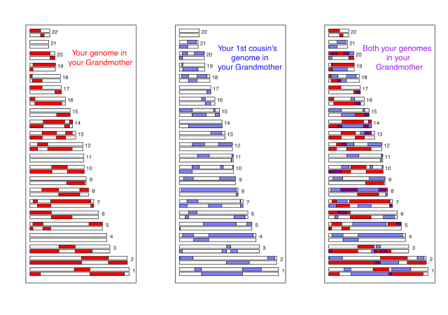
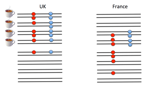
A second major hurdle that we face in understanding polygenic scores is that we do not know the loci that are functionally important for trait variation, only loci that are statistical proxies for them—sometimes called tag SNPs—that will be nearby in the genome. (Technically the SNPs used to construct polygenic scores are in linkage disequilbrium with the functional loci—meaning that genotypes at the tag SNP are correlated with genotypes at the functional locus—but unlikely to be the functional loci themselves.) To understand this point, look at the example below. On the left is a cartoon of people from the UK. Each person has two chromosomes (horizontal black lines) and in this small stretch of the genome there are two loci (red and blue SNPs), the alleles of which are indicated by the presence/absence of a filled circle. Whether an individual drinks a lot of tea is indicated by the tea cup  next to the individual. Both of the filled circle alleles appear to be associated with tea drinking. (Obviously this sample size is laughably small, but you get the point.) However, only one of them is the functional SNP predisposing people toward tea drinking; the other SNP just happens to be associated because the mutation there arose at a similar point in history on the same genetic background. If we guess that the blue allele is the functional one, we would predict that French people have a slightly weaker preference to tea on the basis of this allele. But if we guess the red allele is the functional one, we would predict that the UK and France have very similar tea drinking habits on the basis of this locus.

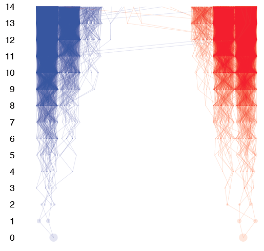
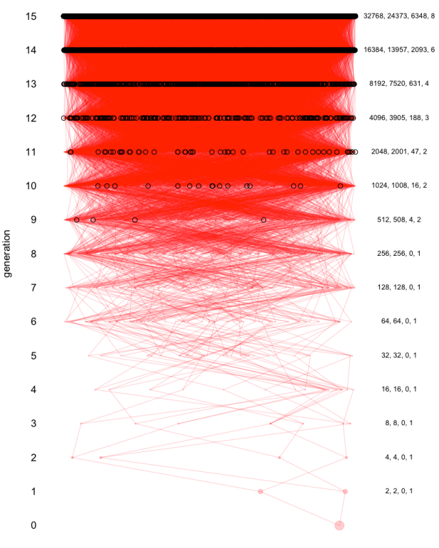
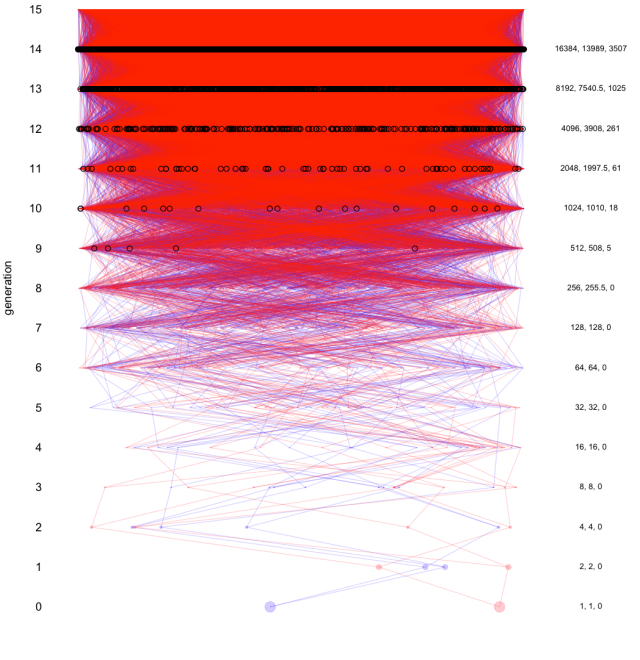
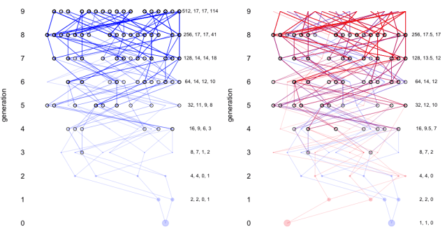
What’s happened here is that the correlation between the alleles at the two loci have changed due to different histories of recombination and genetic drift. Now such a strong change in the correlation of loci is unlikely between two countries, such as Britain and France, that share so much of their genetic history. However, it is a serious problem when comparing populations that have been more distant from each other for a longer period of time. The fact that the correlation between any two SNPs changes over evolutionary time is a major reason why polygenic scores lose predictive ability as we move to populations that have been isolated from each other for more of their history. Even for closely related populations, it may be a problem when we consider that the many weak GWAS signals that likely much of the heritability for typical traits, as these associations may be due to collections of loosely linked SNPs. One way forward would be to perform GWAS in multiple populations and try to narrow down the actual functional SNPs, but again, this is no small undertaking.

tea_LD.png

A second, more subtle force can decrease the predictive validity of polygenic scores. Assortative mating among individuals can drive rapid changes in the SNPs associated with a trait. For example, if people who drink more tea tend to have children with taller people, this pattern of assortative mating can cause greater height and tea drinking to become associated (formally can lead to a genetic correlation). In other words, height-increasing alleles will be associated with tea drinking because the offspring of tea-drinking/tall couples will have alleles associated with both tea drinking and height. Even after assortative mating has stopped, these effects can persist for a few generations, making them potentially hard to rule out.  Such associations need not hold in other populations, however, if they do not have similar patterns assortative mating. Therefore, sets of loci that contribute to trait variation via genetic correlations may change rapidly across environments or populations due to shifts in assortative mating.

We will not map within a single population all of the alleles influencing trait differences among populations.

GWAS have the highest power to map alleles that are present at intermediate frequency in the GWAS population (all else being equal). The functional variants contributing to a trait will differ in frequency among populations due to genetic drift and selection; therefore, GWAS will miss many of the loci contributing to phenotypic variation in other populations. This may not be much of a problem for comparing the UK and French population, as allele frequencies are very similar in the two countries. However, it’s potentially a much bigger problem in comparing more distant populations.

An example of the complexity of the ways in which different variants contribute to a trait in different areas of the world is the genetics of skin pigmentation. The variants that were mapped within European populations, though important in Europe, explain little of the variation in skin pigmentation worldwide. Even variants that explain the lighter European skin pigmentation do not explain the lighter skin pigmentation in East Asians (e.g. see here and here). Work from Sarah Tishkoff and Brenna Henn‘s labs has demonstrated that a number of loci important for explaining skin-pigmentation variation world-wide were  missed by studies focused on non-African populations. A big part of the story was missing until variation within Africa was explored, with undoubtedly much more to uncover about this trait from GWAS in many populations. Furthermore, our understanding of the evolutionary history of skin-pigmentation in Europe has been majorly revised by ancient DNA.  This history of major shifts in our understanding of the genetics and evolutionary history of skin pigmentation suggests that bold claims about other traits, based on incomplete evidence, may well not stand the test of time.

In the coming decade, we will likely uncover a surprising amount of heterogeneity in the alleles controlling trait variation world-wide. Based on genetic drift alone, we should expect as much: the alleles that explain most variance in populations of European ancestry will not be the same alleles in East Asia as allele frequencies drift over time. Also as a result of allele frequency change at many loci, across populations, epistatic relationships among loci may also change in unpredictable ways, confounding cross-population predictions.

These problems of different alleles contributing to  traits in different populations will be compounded for traits subject to natural selection (as well as genetic drift). Whether traits are subject to stabilizing selection or directional selection (shared or divergent), selection will drive more rapid turnover in the loci contributing to trait variation among populations.

Again, one can hope to address these issues by performing GWAS in multiple worldwide populations, but we should expect to have a European-biased view of genetic variation for some time to come, simply because of the size of the studies in these populations dwarfs those done elsewhere.

Conclusion

Undoubtedly the coming decades of human genomics will see breakthroughs in the identification of functional loci, the size of GWAS performed world-wide, and in the statistical methodologies used to understand trait variation. There is also no doubt that we will come to understand much more about human variation. However, our ability to perform GWAS to identify loci underlying variation in traits among individuals vastly outstrips our ability to understand the causal mechanisms underlying these differences. In many cases, genetic contributions may not be separable from environmental and cultural differences. Certainly making a case for the relative importance of genetics in explaining among-population differences will involve a lot more work than simply counting up the number of tea preference alleles in populations and seeing how the averages differ.

These complications notwithstanding, I suspect that over the next decade, we are going to see a lot of partial results and incomplete (and in some cases initially downright incorrect) stories about the genetics of among-population variation in traits. For example, we now think we know something about the evolution of polygenic height scores among European populations. Results in hand allow us to demonstrate that natural selection has likely driven the higher polygenic height scores of Northern Europeans compared to Southern Europeans (Turchin et al, Berg and Coop, Robinson et al Mathieson et al, Berg, Zhang, & Coop). But they do not convincingly demonstrate that among-population differences in height in Europe are genetic (for all the reasons outlined above; for more, see here). Furthermore, our understanding of height genetics drops off quickly as we move away from Europe: we are even further away from understanding height differences among populations across Eurasia, and European-GWAS polygenic height predictions are positively misleading when applied to African populations. The complexity of such partial results reflects our uncertainty about the genetics of height–and that’s for height, an easily measured and well-studied trait. Applied to other and more fraught traits, this patchy understanding of the contribution of genetics to phenotypic differences will be fertile ground for misleading claims.

Finally, there is a more fundamental disconnect between talk of polygenic scores and what some people seem to think they might learn from this kind of research. Even if we could attribute some proportion of the phenotypic difference to a difference in polygenic score, on a deeper level, it is not even clear whether such a result really answers the question that an average person means to ask when they ask whether a difference is “genetic.” Saying a phenotypic difference among individuals is genetic often is implicitly taken as implying that it is immutable or unavoidable. However, even if we could attribute a some proportion of the difference in phenotypes between groups to polygenic scores, it would not lend support to the idea that this difference is immutable or “natural”. That is simply not how genetic variation works, as many phenotypes where genetics plays a role are modifiable.Without at least some working knowledge of causal mechanisms underlying the action of the genetic variation contributing to a trait, we may often not know how environment and culture shape the actions of these variants, nor how changes in these factors may modify any role played by genetics. Even if our tea polygenic scores were strongly predictive within and among populations, would cultural changes, e.g. a Europe-wide health food craze for drinking tea with dinner, stand these results on their head? Will taking tea with a meal moderate the role of caffeine-sensitivity SNPs; will exercise-conscious people now drink more tea? Will we know enough about the interaction of culture and genetics to predict this? If we do not, the statement that a difference in polygenic scores plays a role in explaining a difference in phenotypes among populations may often have little to say about how we as individuals or societies should view that difference. But will these critical subtleties be lost in the public’s understanding of results based on polygenic scores? Will such results be wrongly taken as supporting genetic determinism about human variation?


Posted in popgen teaching, Uncategorized | 4 Comments

Where did your genetic ancestors come from?

[Part of a continuing set of blog posts on genetics and genealogy]
In the last post I described how you are descended from a vast number of ancestors, from all over the world. But how much of your genome traces back to each of these ancestors?

You have two copies of your 22 autosomal chromosomes, one you inherited from your biological mother and one from your father (we’ll ignore for the moment the small subset of our genomes that are inherited in a different manner, i.e., the mitochondria, and the Y chromosome, and the X chromosome). Your mother in turn had two copies of each of these chromosomes; one she received from your maternal grandfather and one from your maternal grandmother. Your mother can only pass on a single copy of each of these chromosome into the egg (though the process called meiosis). When she comes to pass on a particular chromosome, sometimes she transmits you a copy of your maternal grandmother’s chromosome, and sometimes she passes you a copy of your maternal grandfather’s chromosome. In those cases, your entire copy of that particular chromosome traces to your either your maternal grandmother or your maternal grandfather. However, frequently when she copies out her chromosome she takes big chunks* from her mum’s copy and then switches to her dad’s copy. Imagine that each of these chromosomes are books — now you could have inherited page 1-253 from your maternal grandmother and 254-600 from your maternal grandfather. In that way, the copy of the chromosomal book you receive from your mother will be a mosaic of the copies in your maternal grandfather and grandmother. The mosaic you receive was bound together carefully so that you aren’t missing any pages and so you get the entire story (no annoying bits where you’re missing the page where the murderer isnrevealed). The process of forming the mosaic is called recombination, and the switch points in the story are called recombination events (or crossovers).

In the figure below I show a picture of all 22 autosomes, two copies of each. Each chromosome is shown as a long white block, the length of the block is proportional to the length of the chromosome.

parents_grandparents.png

Let’s imagine that the individual is you. The maternal genome (the copy from your mum, note correct spelling on mum) is shown on top, and the paternal genome on the bottom. I paint each chromosome with a colour indicating where an individual’s genetic material has been copied from. So for example, you inherited the entirety your father’s paternal copy of chromosome 21; see how the entire lower, paternal copy of your father’s chromosome 21 is highlighted. So you have none of your paternal grandma’s copy of chromosome 21. Your paternal grandma had a full copy herself (she transmitted her chromosome to her son), but none of that is in your genome, as your father didn’t transmit it to you. Your copy of chromosome 21 from your mother is a mosaic (a recombinant) between her maternal and paternal copies of this chromosome, note how the painting of this chromosome changes from bottom to top as we move left to right along chromosome 21. Going another generation back see how this means that you have inherited the left part of chromosome 21 from your maternal grandma, and the right half of chromosome from your maternal grandfather.

Now let’s track your genome up your male lineage (technically your patrilineage), following your father, your father’s father, etc :

male_line.png

Each generation you go back, you inherit less of your genome from any given ancestor. Six generations back, you only inherited a small section at the tip of chromosome 13, and a section of chromosome 5. By chance, those fragments are both inherited from great-great-great-great-great-great grandfather’s maternal copy of the genome, the one he received from his mother. Thus, moving one more generation back, we find that none of your (autosomal) genome has been copied down over the generations from this male lineage. The entirety of the two copies of your genome is present back then, scattered across your sixth four ancestors, it just happens that none of it is derived from this individual. Despite being your genealogical ancestor, he is not your genetic ancestor, none of their story has been passed down to you. If you are female none of your genome descends from him, if you are male you will have his Y chromosome but your daughters will have nothing from him. Your ancestor had a full genome, and they transmitted their genome to their children, and their children in turn transmitted some of it to their grandchildren, but over the generations it was whittled down till by chance none of it is in you. His genomic story may live on in some of his other descendants, e.g. your sixth cousins, but not in you.

In the figure below I show a simulation of how much of your autosomal genome is present in each genealogical ancestor as we go back up the generations.
genetic_pie_2.png
[discussed in more detail here]
Your genome is shown in the middle, in the next semi-circle out are your two parents (blue and red), then your four grandparents, and so one as we move out. At each level, the intensity of the colour indicate how much of your autosomal genome is in that ancestor, the total contribution to your genome sums to 100%.
For the first number of generations, all of your genealogical ancestors are your genetic ancestors, and contributed big chunks of your genome to you. But as we go further back we start to run into ancestors who contributed no genetic ancestry to your genome (these individuals are indicated by the white spaces). For example following the male lineage of fathers’ lineage back on far right, marked with an blue arrow; there, seven generations back, is that first ancestor who contributed nothing to your autosome. Moving back through the generations, more and more of your ancestors do not contribute to you genome”. Your family tree is soon full of genetic holes, ancestors who contribute no big regions of your genome to you, see how more and more of your ancestors are coloured white as we move out through the semicircles. Below I show the rapid increase of your number of genealogical ancestors (red line 2k) contrasted with your number of genetic ancestors (black dots), which grows far more slowly:

num_genetic_ancs.png
Your genetic ancestors rapidly become a tiny fraction of your total number of ancestors. The probability that you inherit genetic material from an ancestor drops off rapidly as we move back over the generations. I discuss these ideas in more depth here and here.

In the last post, I described how your vast number of ancestors meant that you were descended from nearly everyone in the world more than a few thousand years back. But you are only a genetic descendant of a relatively few of those individuals, as most have left no trace in your genome. For example, you might be able to trace a particular route through your pedigree to Charlemagne, as can almost any one with European ancestry, but there’s less than a 1/100 million chance that you’re a genetic descendant of Charlemagne due to that particular connection through your pedigree. Forty generations back most of your genome traces back to a random subset of around twenty-six hundred individuals out of all your millions of ancestors. It’s unlikely that Charlemagne is one of them.

While your family tree is staggeringly vast and geographically widespread, your genetic ancestry is likely more restricted. To illustrate this, consider the simulation shown in the gif below. Similar to those pictures in the last post, I trace back your ancestry over the generations. But now I’ve coloured genealogical ancestors in red, genetic ancestors are overlain in blue.

ped_5_output
The x axis gives the geographic location of the ancestor. I’m simulating a population of 500,000 individuals spread out over 50 geographic regions. The vertical lines give the boundaries between these regions. Each generation back an individual’s parent comes from a neighbouring region with a 25% probability, and from a randomly chosen region with a 1/50 probability. Each time the gif ticks over, the histogram shows you how many ancestors you have in each region that number of generations back.

Up to about 7 generations back all of your ancestors are genetic ancestors (the blue perfectly overlays the red, but soon after that many of your ancestors make no major genetic contribution to you. In the figure below I show a zoomed in histogram of the geographic locations of ancestors in a simulation 17 generations back
zoom_in_17_gens.png
You soon have genealogical ancestors from all over the place, yet there are geographic regions in which you have no recent genetic ancestors. Some of your genetic ancestors are from distant locations, but most are much more geographically restricted. That’s because the majority of routes back through your family tree trace back ancestors who stayed closer to home.

A thousand years back I’m descended from nearly everyone everywhere in Europe. I’m related to these individuals via millions of lines of descent back through my vast family tree. Yet the majority of the lines back through my pedigree trace to people living in the UK and Western Europe. Many lines trace back to more distant locations, but these are relatively few in number compared to those tracing back to closer to home. Ancestors along each of these lines are (roughly) equally likely to contribute to my genome. Therefore, most of my roughly 2600 genetic ancestors from 1000 years ago, who contributed the majority of my genome to me, will be random people living in the UK and western Europe at that time (who happened to leave descendants).

Looking back a few thousand years more, I’m a descendant of nearly everyone who ever lived almost everywhere in the world (at least those who left descendants, and many did). Yet most of the just over ~6000 individuals from that time who contributed the majority of my genome to me will mostly be found all over Western Eurasia. There’s nothing much special about these individuals who happen to be my genetic ancestors a few thousand years back. They’re likely not royalty. My genetic ancestors are just a random subset of all of my genealogical ancestors, they just happen to be my genetic ancestors due to the vagaries of meiosis and recombination.

This fact also means that my set of genetic ancestors, say a thousand years ago, likely doesn’t overlap much with yours, even if you’re from the UK. However, my genetic ancestors will overlap with some (random subset) of the people currently in the UK (and Western Europe). This is why reputable genetic ancestry companies can tell you something infortmative about where your ancestors lived in the past. When 23&me tells me that most of my genetic ancestry traces back to the UK, they’re telling me where the bulk of my ancestors lived, a few hundred to a thousand years ago, even though I have ancestors all over Europe. Although honestly I think they should also phrase this as something like: “the majority of individuals who are Graham’s eighth through sixteenth-cousins currently live in the UK”. That phrasing is much closer to what they are really doing when they look at your genome. Should I be excited if a genomic ancestry company tells me that a few megabases of my genome traces back Scandinavia? Should I start to imagine that my ancestors were Vikings sailing the seven seas? Well, I already knew that my ancestors lived all over Europe, and so I already knew that my ancestors included many Vikings. These genomic connections can be fun, but if I have Scandinavian genomic ancestry and someone else in the UK does not, that does not mean that I can claim they do not have Viking ancestors, nor that I’m more Viking than they are. Such differences are more likely the result of the randomness of meiosis than an excess of berserker blood in your ancestors.

Does it matter that I’m not genetically related to all of my ancestors? In talking about these topics I’ve been told things like “I won’t bother tracing my family tree back more than eight generations, as I guess many of those people aren’t my ancestors”. But any individual to whom my family tree traces back is my ancestor. My great^8 grandmother had a profound influence on who her son (my great^7 grandfather) was, and she shaped who many of my ancestors were. Her genomic story was passed down to my grandfather and father. The fact that my father, due to the randomness of meiosis and recombination, did not pass on the small part of his genome that he had inherited from her, to me seems largely irrelevant. Even if I inherited a small fraction of my genome from her, it would mean little in terms of how I resemble her. She is just one of the hundreds of genomic book passages that may been passed down from my ancestors in her generation.

Looking further back still, some sixty thousand years ago modern humans interbred with Neanderthals (and Denisovans) as our ancestors spread out of Africa. Note that I did mean to say“our ancestors”, as in, absolutely everyone’s. Everyone in the world is descended from those modern humans who first met and mated with Neanderthals, just as we are all the descendants of the many groups of people who remained in Africa. If we look carefully, using computational tools that detect subtle genomic signals, I can see that around 2% of my genome traces back to Neanderthal ancestors (this 2% of Neanderthal ancestry is scattered all over my genome like Neanderthal confetti). If you have a lot of Sub-Saharan ancestry, we would likely detect many fewer Neanderthal blocks of ancestry in your genome. You’re still descended from Neanderthals, but fewer of the routes back through your family tree trace back to Neanderthal than through mine. The fact that any of us carry the genomic trace of Neanderthal interbreeding is a fascinating insight into all of our family trees, and one of the most surprising findings in human genomics in the past decade. That this Neanderthal ancestry isn’t evenly split over everyone in the world is a statement that we vary in our degree of relatedness to people who lived tens of thousands of years ago. But this variation in our pedigrees are quantitative rather than qualitative; we are bound together much more by our vast shared family tree than we are divided by it.

These ideas are sometimes deeply unintuitive. I’ve studied them for over a decade and still truly cannot really get my head around how I can be descended from so many people, and yet genetically to so few of them, just a few thousand years ago. However, grappling with these ideas is important. All of us will have to get much more used to thinking about these ideas of genomics, ancestry, and family trees. Millions of people have chosen to be genotyped for ancestry tests, many more are being genotyped as part of large panels for medical genetics research. What genomics can and cannot say about our family history will become much more central to how we perceive ourselves over the coming decade.

In the coming posts we’ll bring into focus more seemingly contradictory ideas. We’ll see that despite the fact that everyone is related just a few thousand years back, I have to go back over a hundred thousand years to find the common ancestor of all of our mitochondria. Even more surprisingly, we’ll see that the copies of a chromosome I have from mother and father last share a common ancestor more than half a million years ago.
____________________________________________________________

*What I’m describing here is the recombination process of crossing over. You will also inherit small stretches of DNA from either parent due to gene conversion. You can think of gene conversion as your mum switching from copying out her mother’s (your maternal grandmother’s) copy of chromosome 21 to copying from her father’s (you maternal grandfather’s) copy for a short stretch. There’s more of these gene conversions per meiosis than crossover (~300 hundred compared to ~30 on average). However, these gene conversion events are just short stretches of copying, just a few hundred letters (bases) long, while crossovers demark switches between long stretches of copying between the parental chromosomes (for 100s of millions of bases). Therefore, crossovers determine the bulk of your ancestry. That said these gene conversion events do mean that you have more genetic ancestors than the numbers above would indicate, here’s the graph from above with genetic ancestors due to both gene conversion and crossing over:
Genetic_ancs_inc_gene_con.png
Your number of genetic ancestors including gene conversion keeps up with you genealogical common ancestors for long than the number of genetic ancestors tracking crossovers alone. However, these extra recent genetic ancestors due to gene conversion contribute very little to your genome. For example, 14 generations back you you have an extra ~7000 genetic ancestors due to gene conversion, compared to the ~950 due crossover alone. But each of these extra “gene conversion” genetic ancestors contribute only a few hundred bases to you, while the ones due to crossovers contribute several million bases. Less than 1/5000th of your genome traces back to all of these gene conversion genetic ancestors combined 14 generations back. Therefore, through the post I’ve ignored these extra gene conversion ancestors, and framed it as where most of your ancestry traces back to (note the use of weasel words like “most”, and “little to none”). I think that is a more accurate reflection of where your ancestry traces back to, but I did struggle a bit with how to simplify these complex ideas.

Posted in genetic genealogy, popgen teaching | 14 Comments

Your ancestors lived all over the world

In the last post I discussed the idea that that we are all related in the recent past (building off the work of Chang, Derrida, and colleagues). This idea can be confusing; for many of us our ancestors all seem to come from one or a few geographic locations. How does this geographic restriction affect the relatedness between modern day humans?

I’m originally from the UK, but I’ve been in the States for a third of my life. However, in general my ancestors weren’t big travelers. My family is from Yorkshire and Staffordshire in England. My mum traced our family tree back a few years ago; my photocopy of it is stuffed in a drawer somewhere. A bit further back, apparently many generations of my granddad’s side of the family are buried in a churchyard in a village (I think) somewhere outside of Melton Mowbray. No seafaring life with a kid in every port for my ancestors. Unsurprisingly then my ancestry report from 23&me makes for dull reading, and says my recent ancestry is all from the UK. How then do I have ancestors all over the world just a few thousand years back? Is it really possible that I am related to nearly everyone who lived in the entire world?

The key to this is that I, and you, have vast number of ancestors just a short time into the past. Fourteen generations back –roughly four hundred years ago– you have over sixteen thousand ancestors. Twenty generations back you have (potentially) over million different people as ancestors. Even if only a few people in the past emigrated from a specific country to the country you’re from, you are likely descended from those immigrants.

To illustrate this, consider the following simulation. We track your ancestors back over the generations as we did before. But now instead of coming from a well-mixed population, I’ve divided up the population of a million individuals into ten regions. These regions are arrayed along a line for simplicity, and the boundaries are shown as vertical lines. Each generation back, there’s a 1/50 chance that an individual’s parent comes from a neighbouring region. We see our first local migration event 4 generations back; one of your 16 great-great-grandparents is from the neighbouring region. See how their pedigree in that region rapidly expands; you soon have many ancestors in this second region.

Screen Shot 2017-11-27 at 7.04.03 PM.png

On top of the local migration, in these simulations there’s a 1/5000 chance that an individual’s parent comes from some more distant region (chosen at random). We only see these long distance migrants deep in your pedigree. These migration events are occurring in the population all the time. However, It’s unlikely that any of your recent ancestors is one of these immigrants, as there’s only a low rate of immigration. But you have vast numbers of ancestors further back, and so further back you start to be descended from them too. See how eleven generations back you have over two thousand ancestors, and a couple of them are from distant regions. Looking slightly further back, each of your immigrant ancestors has many ancestors from his or her distant homeland. You’ll soon be descended from nearly everyone in these distant regions.

This rapid spatial expansion of your ancestors means also that you share recent genealogical ancestors with present-day individuals in distant locations, as both your and their ancestors are found all over the place. To illustrate this, I’ve run our simulation for another individual who lives at the other end of the set of regions from you. Below I plot your two family trees together.

Screen Shot 2017-11-27 at 7.06.22 PM.png

Maybe you think 1/5000 individuals being an immigrant from some distant location is too high, and it likely is for distant locations or other continents. However, even if it were as low as 1 in a million, we only have to go back roughly 600 years to find you descended from one of these rare long distant immigrants. A thousand years back I’m descended from nearly every traveler of the high seas who set foot in Europe. Well at least those that left descendants there; if they had an unfortunate accident with a short-sword before conceiving a child, then they’re out of luck. As a result of the ones who had kids, I have millions of ancestors on every habitable continent just a few thousands of years ago.

I’m not an anthropologist of distant oceanic islands, so I can’t tell you for sure that there’s nowhere in the world so remote (and so long isolated) that we can rule out that you recent shared ancestry with people from these remote regions. However, I can confidently tell you that you’re related to nearly everyone in the world via ancestors just a few thousand years back. Even for the remotest locations in the world, I suspect that they too are soon part of our family tree. as nowhere has been completely isolated for many thousands of years.

Some links to related topics:

Simulations
by Brian Pears of the spread of ancestors across the UK.

Kaplanis et al (page 6) from Yaniv Erlich’s group explore patterns of dispersal using vast human genealogies. See a video of their graphic depiction of dispersal here.

Jerome Kelleher et al explore technical aspects of the spatial spread of your ancestors, and calculate the rate of spread of the rapidly expanding geographic region your ancestors are drawn from. We’ve used related ideas to calculate dispersal distances from genetic data (see Harald Ringbauer et al.).

Thanks to Vince Buffalo, Doc Edge, Emily Josephs, and Jeff Ross-Ibarra for feedback on an earlier draft of this post.

Posted in genetic genealogy, popgen teaching | 2 Comments

Our vast, shared family tree.

You might not like to admit it, but you’re related to me.

It’s very unlikely that you’re my sibling (I’m not even sure if my family read these posts). You’re one of over seven billion people alive today, and I have only one sister, so the chance that you as a random person are my sibling is < 1 in a billion. You're not my first cousin, because (as far as I know) I dont have any first cousins. But further back than that it all starts it go a bit hazy. I have eight great-grandparents and I vaguely know their names and know some of their descendants, I'm guessing you're not one of them (I met some of my 2nd cousins once at a Christmas long ago). But how far do I have to go back till I find I'm related to you? I have sixteen great-great grandparents, I have no clue who they were, and I certainly have no clue who my third cousins are. My number of ancestors doubles every generation I go back, as does yours. And my awareness of who these ancestors were, and my distant cousins, drops even more quickly.

Our numbers of ancestors grow so quickly that it is soon unavoidable that we have shared ancestors. Six hundred years ago (roughly 20 generations back) I'll have just over a million ancestors alive (220), a thousand years back I potentially have over a billion ancestors alive (233). There simply aren’t that many people alive in Europe back then, and so I’m a descendant of everyone who lived then as long as they left descendants (and vast numbers did). So I’m related to everyone famous who lived back then, and everyone non-famous as well. If you have European ancestry, you’ll be related to them all too, and we’ll be distant cousins.

To illustrate this idea consider the following computer simulation. Let’s think of a constant size population of one hundred thousand people. I’m in the present (the red dot), Each generation back my ancestors are drawn at random from the one hundred thousand people. Just for display purposes, I’ve arrayed the hundred thousand people out on a horizontal line, representing the population. Each generation back I draw lines from my ancestors in that generation to my ancestors one further generation back. You can see the lines tracing from my parents, to my four grandparents, and so on. The number of lineages of my family tree that we’re tracing quickly gets mindboggling, and we cant see individual connections anymore.

Screen Shot 2017-11-14 at 3.04.04 PM.png

Every time an ancestor appears more than once in my simulated pedigree I draw a circle around them. I’ve kept track of (left to right) my number of unique ancestors in each generation, the number of ancestors that are present more than once in my pedigree, and the maximum number of times an individual appears in my pedigree. My first overlapping ancestors occurs nine generations back; I should have 512 ancestors, but I have 508 ancestors instead. Four individuals are circled, each of them are my great7 grandparents twice over (technically these are called inbreeding loops). I can trace back multiple routes through my pedigree which lead to each of these ancestors. By fifteen generations back I should have over thirty two thousand ancestors, but in fact I only have less than twenty five thousand ancestors, there’s roughly six thousand individuals who appear in my pedigree more than once in that generation. One of them appears several times over. My pedigree is collapsing in on itself.

Now lets think about the overlap between our family trees. I’ve drawn your (simulated) pedigree back in blue, with mine overlain. When I find an individual who is a new genealogical ancestor to both of us I draw a circle around them. I keep track of the number of shared ancestors (the rightmost number, the other two give 2k and the mean actual number of ancestors a modern individual has). We don’t have to go very far back to find that our family start to overlap.
Screen Shot 2017-11-14 at 3.12.37 PM.png

It’s also fun to do these simulations with small population sizes (see below). Here I do them, with only 20 individuals. Obviously this population size is pretty unrealistic, but it does allow you to see the overlap in the pedigrees more clearly.
Screen Shot 2017-11-15 at 7.07.56 PM.png

The pedigree collapse problem has been highlighted by many people over the years, both for real pedigrees and through mathematical models. A good popular account of pedigree collapse is found in the New Yorker article the Mountain of Names (and the book of the same name). Also Carl Zimmer and in Adam Rutherford’s book both have great accounts of these ideas, and their genetic implications. There’s a nice article on the math underlying pedigree collapse by Wachter, describe the number of unique ancestors of person of British ancestry at the Norman Conquest (I’ve posted a [bad] pdf of the chapter here).

Chang extended these ideas and explored how far back we have to go to find the first common genealogical ancestor of the entire population, i.e. the first individual who all of our family trees trace back to, in a well mixed population of size N individuals. He found that we should expect to find the common ancestor of the entire population roughly log2(N) generations in the past, and that there’s little randomness in this result (i.e. if we run the process multiple times we get very similar answer). The math of this is somewhat involved, but intuitively the answer depends on the logarithm of the population size in base two, because you number of ancestors grows as 2k, so number of ancestors will be roughly the population size when 2k=N, which we can rearrange to find that the critical time should be roughly k=log2(N) generations in the past. He showed that (in a well mixed) population with N individuals, we only have to go 1.77 log2(N) generations in the past to find the time when everyone in the population (who left descendants) is an ancestor to the entire population.

Rhoade, Olsen, and Chang showed that even considering the low levels of migration among world-wide populations you only have to go back a few thousand years to find the first common genealogical ancestor of all humans. And we dont have to go much further back in time to find that everyone in the world (who left descendants) is an ancestor of everyone in the present. Even quite high levels of inbreeding make little difference to these results (see Lachance’s paper). This idea is wild to think about, we’re all descended from everyone in the world (who has descendants) more than a few thousand years back. Your family tree is vast and vastly messy, no one is descended from just one group of people.

A range of other people have worked on this problem. Notably Derrida, Manrubia, and Zanette have studied the number of times ancestors in pedigrees in mathematical models (see also their followup paper). They also showed that roughly 80% of individuals in a given generation (further in past than the cut off given by Chang) can expect to be ancestors of the entire population today. And Manrubia, Derrida, and Zanette have also written a nice, reasonably accessible account of many of these results and more.

In the next post we’ll turn what this implies about how genetically related we are to other people. We’ll address why, even though we are all very closely related, we aren’t genetically identical to each other. We’ll see, somewhat paradoxically, that some of the differences among humans, even within populations, are millions of years old. We’ll talk about why, even though we all have Neanderthal ancestors only some of us carry traces of Neanderthal ancestry in our genomes.

The code for these plots is on github here. I wrote the code, and most of this blog post, over a couple of our toddler’s naps while sat in a gravel pullout by a lake (he only naps in the car). It’s a nice lake, see the pic below, but I get some funny looks from cyclists as they bike past and watch me typing. This is all the say, that the code and blogpost are quickly (and somewhat poorly) written.

DMOlTrFUQAAf6Cg.jpg

Posted in genetic genealogy, popgen teaching | 5 Comments

Genomics of Isolation by distance in Florida Scrub Jays

Stepfanie Aguillon and Nancy Chen‘s paper on combining genomics and genealogy to study isolation by distance is out in PLOS Genetics.

PLOS_cover_image.jpg

Posted in Uncategorized | Leave a comment

Coop lab talks at Evolution 2017

Emily Josephs “Detecting polygenic adaptation in maize” 9am, Sunday, b117_119.

Gideon Bradburd. “Isolation by distance as a null hypothesis of population structure” Sunday, 9:00AM-9:15AM Oregon Ballroom 204. “ASN Spotlight Symposium- Processes underlying pattern: considering the evolutionary mechanisms underlying population-level differentiation”

Nancy Chen: Detecting short-term selection in a pedigreed natural population.  Sunday. 4:00 PM – 4:14 PM In session: Contemporary evolution 2. room C123.
Kristin Lee. “Distinguishing among modes of convergent evolution using population genomic data” Sunday, 3:45 PM – 4:14 PM. Oregon ballroom 202. SSB Symposium – Phylogenetic approaches to connecting genotypes to phenotypes 2
Vince Buffalo: “The Temporal Signature of Linked Selection.”  Monday 9.15 AM-9.30AM Population genetics: inference of selection 2.  B114-115
Erin Calfee “Detecting selection for ancestry in admixed populations with arbitrary population structure.”  2:15 Monday. Pop gen: Theory and methods. Room B114-115
Sivan Yair: “Characterizing adaptive Neanderthal introgression in modern humans” 6:30pm. Poster session: population genetics: theory and methods
Posted in cooplab, meetings | Leave a comment

Guest lecture on archaic genomics

Had fun giving a guest lecture in TIm Weaver’s Anthro. course on Neanderthals, pdf of slides here:

Neanderthal_genomics_lecture_Weaver_class

Graham

Posted in popgen teaching, teaching | Leave a comment